K-Armed Bandit Experiments Part 1

K-Armed Bandit Experiments Part 1#

TLDR

For k-armed bandit problems, we see the importance of balancing exploration and exploitation. Just because we found a good action, doesn’t mean we should stick to it. We should allocate some time to explore the rewards from less observed actions that could potentially give us higher rewards!

What’s the K-armed bandit problem?

K-armed bandit problems are the simplest reinforcement learning problems. The idea is there is a set of K distributions of rewards. This distribution is unknown the the RL agent. The goal is to maximize the rewards by sampling from each distribution, much like pulling the lever of the slot machine. Except in this case there are K slot machines, and the distribution of possible winnings in each slot machine are different and unknown. The RL agent must therefore infer the distributions as it plays the game. Note that it’s possible that each of the K distributions change over time. In this case, the agent must be able to adapt to this.

Here, we experiment on the K-armed bandit problem.

Stationary vs non-stationary rewards

We generated K randomly-generated Gaussian distributions of rewards, where the standard deviation is 1 and mean is taken from a Gaussian of 0 mean and 1 standard deviation. We then consider two cases:

Stationary rewards: the reward distributions do not change over the course of the game
Non-stationary rewards: the reward distribution means gradually change via random walk where the changes are sampled from a Gaussian with mean 0 and standard deviation 1.

Four kinds of bandit algorithms

We explore four kinds of bandit algorithms:

Greedy with sample-averaging
Greedy with weighted averaging
Epsilon-Greedy with sample-averaging
Espilon-Greedy with weighted averaging

Sample-average? Weighted average?

Sample-averaging simply means, our estimate of the expected value of each distribution is a simple mean of the collected datapoints about that distribution:

\(Q_{n+1} = \frac{1}{n} \sum_i^n{R_i}\)

Which is equivalent to

\(Q_{n+1} = Q_n + \frac{1}{n}(R_n - Q_n)\)

Meanwhile, weighted averaging means that we place more importance on the more recent rewards in anticipation of changing distributions. The estimate of the value follows an exponentially decaying average:

\(Q_{n+1} = (1-\alpha)^n Q_1 + \sum_i^n{\alpha (1-\alpha)^{n-i}R_i}\)

Which is equivalent to

\(Q_{n+1} = Q_n + \alpha(R_n - Q_n)\)

\(\alpha\) is a fixed “step size” parameter in contrast to sample-averaging where effectively \(\alpha = 1/N(a)\) where \(N(a)\) is the number of times action \(a\) is selected as the game progresses.

Note that for our experiments, we start with an initial Q estimate of 0 for all actions.

Greedy? Epsilon-Greedy?

In these methods, we estimate the expected value of each of the K distributions from our experience while playing the game. We then choose the action as the one that is associated with the distribution of highest estimated expected reward, which mathematically means,

\(a = \text{argmax}_aQ(a)\)

This formulation is called Greedy, where always the action or “arm” in the case of K-armed bandit with the highest estimated expected reward \(Q\) is chosen. However, a modification of this is called Epsilon-Greedy or \(\epsilon\)-Greedy where at any timestep, there is \(\epsilon\) probability of choosing a random action with equal probability and \(1-\epsilon\) probability of a greedy selection.

Exploitation vs Exploration

When we select a greedy action, we call this “exploitation” because we are maximizing our existing knowledge. Meanwhile when we select a random action regardless of past rewards, we call this “exploration” because we are exploring potentially better actions than what we have observed. There is a trade-off between these two because for a given model, it cannot explore and exploit at the same time.

When the model exploits, it is maximizing rewards from more certain actions at the expense of losing opportunity to try potentially better actions. When a model explores, it looks for potentially good actions but miss out on the opportunity to maximize more certain good actions, while also exposing itself to risk of lower rewards.

Experiments#

We summarize below our experiment parameters. There are k_arms arms or distributions of rewards. Each game has steps timesteps. For our analysis we run n_trials trials or independent runs of the game, the results of which we average. The standard deviation for sampling how much we change the means of the K reward distributions for the non-stationary problem is some value q_delta_std.

k_arms = 10 # number of levers / arms
steps = 2000 # count steps in an episode
n_trials = 2000 # number of independent runs/trials
q_delta_std = 0.1 # standard deviation of the Gaussian used for random walk on the true q() values

Stationary Problem#

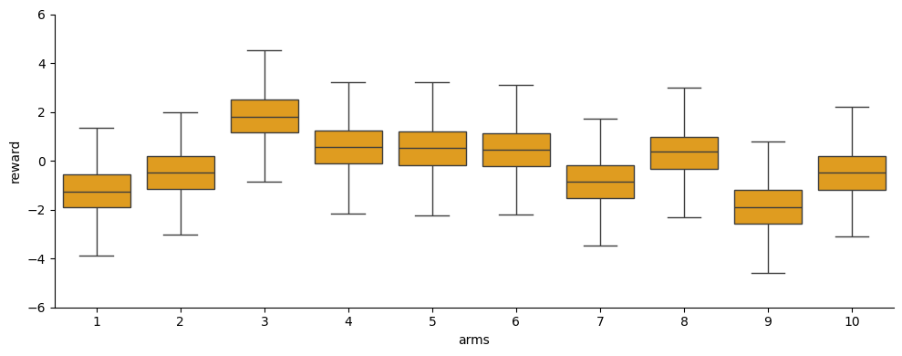
Below is an example of K randomly generated distributions of rewards for the K-armed bandit problem with fixed reward distributions.

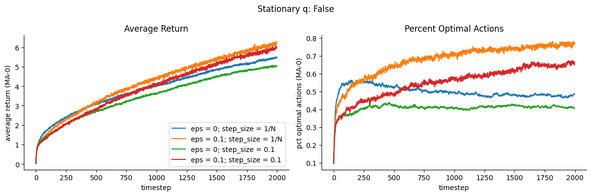
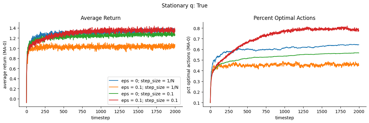
../_images/f2a0dc2debaa6c226968b98777fdec9e42c28ca97f53f3e1b59f5f7b5d02614b.png

For this stationary reward problem, we show to the left below the average reward over timesteps for the different algorithms. Here eps=0 means Greedy, and eps=0.1 means Epsilon-Greedy. step_size = 1/N means the algorithm uses sample-averaging, while step_size = 0.1 means the algorithm uses weighted averaging with \(\alpha = 0.1\)

To the right, we show the proportion among all trials that the optimal action (corresponding to the highest true expected return \(q(a)\)) was selected.

Observations

Best performers
- Epsilon-Greedy with weighted averaging (red) which also got the highest percent optimal actions
- Greedy with sample-averaging (blue)
Worst performers
- Greedy with weighted averaging (green)
- Epsilon-Greedy with sample-averaging (orange)

Questions (I don’t know the answers to yet)

For Greedy, why does weighted averaging worsen performance while sample averaging improves performance?
For Epsilon-Greedy, why does weighted averaging improve performance while sample averaging worsens performance?

../_images/abd7ad536731e94f27004ddf9f41c0109b16a8e76239ae441c0849350b7af71d.png

Non-stationary Problem#

We show in the animation below an example of K randomly generated distributions that gradually change means over the course of the game.

<Figure size 640x480 with 0 Axes>

We show below the results for the stationary reward problem.