k-Fold Cross-Validation Experiments

k-Fold Cross-Validation Experiments#

November 6, 2024

TLDR#

Validation and k-fold Cross Validation are gold standard for getting a sense of test performance as well as for model selection or hyperparameter tuning.

However, we have to be aware of some of their pitfalls. We can look at it through the context of the bias-variance trade-off.

In the case of datasets with outliers or “high leverage” points, simple validation splits may lead to a bias (the expected validation set error tends to overestimate the test error) but also a high variance (the values of validation errors across many trials are widely different). This has implications in hyperparameter tuning where a simple validation split may yield inconsistent sets of optimal hyperparameters.

However, when outliers are not present, simple validation yields consistent results.

Meanwhile k-fold CV also has bias, tending to also overestimate the test error, but has much lower variance, yielding much more consistent results than simple validation. Hence, k-fold CV does seem to be a much more reliable approach to hyperparameter tuning than simple validation.

Take-away: use k-fold CV as much as possible. Simple validation splits will tend to have high variance in its estimates when outlier or high leverage points are present. Alternatively, manage outlier or high leverage points by scaling or removing them altogether prior to validation split evaluation.

k-Fold Cross Validation#

When selecting models or model hyperparameters, we wish to ideally select based on which model performs best on all possible values of the data. However, usually, we are only given training data, which do not cover the full support of our data distribution. k-Fold Cross-Validation (k-fold CV) is a technique for estimating the error we expect on data that go beyond the training data (which we’ll call test set) but still come from the same distribution of the training set.

However, because of the way k-fold CV works (which is you shuffle then split into k-groups), it’s possible this becomes problematic for estimating the test performance (or error) when we have rare extreme values of input \(X\) (high leverage datapoints) that result in extreme values of response \(Y\) (outliers). We will use “high-leverage points” and “outliers” interchangeably.

Violation of the iid Assumption#

k-fold CV splits the training data in a way that violates the iid (independent, indentically-distributed) assumption when we estimate the error, e.g. MSE. Why? Because it splits the data into k-folds without replacement. And putting high leverage/outlier points in one validation fold/group essentially removes the probability it gets selected for the other folds. This could potentially limit its applicability as an estimator of test set error.

Synthetic Dataset#

To test our speculation, we experiment on a synthetic dataset of the form

\(Y = \beta_0 + \beta_1 X_1^2 + \beta_2 X_2^2 ... + \beta_p X_p^2 + \epsilon\)

where \(\epsilon\) is an independent error term taken from a normal distribution \(N(0, 1)\). Why square the predictors instead of just keep it linear? Making it a simple linear sum will make the problem trivial for a linear regression model, which is the model we use in these experiments. We want to fit a linear model on this quadratic function.

To add high-leverage / outlier points, we randomly select a proportion of samples for each predictor independent of other predictors. Then we multiply those values of \(X_j\) by some multiplier. The responses \(Y_j\) are simply computed using the quadratic model defined above.

We generated 1 million datapoints, 10,000 of these were randomly selected for the train set, while the rest were used for the test set.

Experiment Setup#

We first checked the reliability of k-fold CV on this dataset. We chose \(k=100\). We shuffled the train data, then we split into 100 folds/groups. Then we apply k-fold CV, getting a total of 100 MSEs. We then compute the mean of these MSEs and that becomes the k-fold MSE estimate. But we are not concerned with this particular estimate. We are concerned with the reliability of k-fold CV as a method, so we run 100 trials of 100-fold CV. Each trial we get the mean MSE, each of which is an estimate of the test MSE,

\(\hat{\text{MSE}} = \text{mean}({\text{MSE}_{k}}) \approx \text{MSE}_{test}\).

Results#

We then analyzed the mean and standard deviation of these estimates and found that the standard deviation of the estimate is low and \(\text{mean}(\hat{\text{MSE}}) \pm \text{std}(\hat{\text{MSE}})\) does not cover the ground truth test MSE. The ground truth test MSE is computed by fitting on the entire train set and testing on the test set.

We find that \(\hat{\text{MSE}}\) has low variance as an estimator, so running different trials of k-fold CV will more or less yield the same result. So while we will rarely have a case where we will more closely match the \(\text{MSE}_{test}\), the consistency of the results is an advantage of k-fold CV in this case.

We then speculated an alternative method that does not suffer the iid violation of k-fold CV. The approach is we simply do a simple validation split, but do it 100 times which we’ll call “fold” for consistency. Each time, we shuffle the data and split into 99% training and 1% validation. This no longer violates the iid assumption because each fold does not rob the other folds of the possibility of picking particular datapoints. We then get the mean of the 100 MSEs. Then again, we are concerned with the reliability of the approach, so we ran 100 trials, with each trial computing the mean of 100 MSEs. We then analyzed the distribution of MSEs and found that the \(\text{mean}(\hat{\text{MSE}}) \pm \text{std}(\hat{\text{MSE}})\) now captures the ground truth test MSE.

However, the new approach has an increased variance such that running any of this 100-“fold” validation to estimate \(\hat{\text{MSE}}\) will more likely yield much more varied results.

We tested on the more realistic 10-fold and 5-fold CV and we get similar results.

In the absence of outliers, the two approaches still more or less have the same \(\text{mean}(\hat{\text{MSE}})\) which overestimate the ground truth \(\text{MSE}_{test}\). But the standard deviation (relative to the mean) of the second approach is much lower when there are no outliers vs when there are outliers.

Using k-Nearest Neighbors (kNN) regression to investigate the reliability of these two validation approaches to finding the optimal \(k\), we find that when the data does not contain outliers, the second approach where we do simple random validation T times seems marginally more reliable than k-fold CV. However, we find that in the presence of outliers, simple validation yields high variation in the \(\hat{\text{MSE}}\) vs \(k\) charts and yields high variation in the selected optimal \(k\).

Some Questions#

We find that it seems k-fold CV has low variance, even if it’s far from the true test MSE. Doing simple validation many times and averaging the results yield similar results as k-fold CV but with higher variance. What’s the explanation for these?

We’re not sure how general these results are or if there are flaws in how we set up these experiments.

Experiment Details#

We define our function as a linear model of \(X_j^2\) predictors with some random noise. In this toy example, we sample the ground truth coefficients from a normal distribution, and we sample \(X\) from a normal distribution as well. A certain proportion of each predictor \(X_j\) is independently chosen and multiplied by a multiplier to serve as high leverage data points.

import numpy as np
import matplotlib.pyplot as plt

# define a ground truth generative function
def gen_func(n=1000000, n_predictors=5, p_leverage=0.001, mult_leverage=10, seed=42):
    np.random.seed(seed)
    coeffs = np.random.normal(0, 1, size=n_predictors)
    X = np.random.normal(0, 1, size=(n, n_predictors))

    # for each x_i, we randomly select p_leverage% and multiply by mult_leverage
    inds = np.random.choice(range(X.shape[0]), (int(X.shape[1]), int(X.shape[0]*p_leverage)))
    X[inds] = X[inds] * mult_leverage

    Y = 10 + X**2 @ coeffs + np.random.normal(0, 1) # make it squared
    return X, Y, coeffs

We generate 1 million datapoints from our generator. 10,000 are randomly selected to be the training data (from which we will derive the validation sets as well)

def gen_train_test(N, N_train, **kwargs):

    X, Y, coeffs = gen_func(**kwargs)
    inds = np.arange(N)
    np.random.seed(42)
    np.random.shuffle(inds)
    inds_train = inds[:N_train]
    inds_test = inds[N_train:]

    X_train = X[inds_train]
    Y_train = Y[inds_train]

    X_test = X[inds_test]
    Y_test = Y[inds_test]

    print("Coefficients:                ", coeffs)
    print("len(X_train), len(X_test):   ", len(X_train), len(X_test))
    print("len (Y_train), len(Y_test):  ", len(Y_train), len(Y_test))

    return X_train, X_test, Y_train, Y_test

N = 1000000
N_train = 10000
kwargs = dict(n=N, n_predictors=5, p_leverage=0.0001, mult_leverage=10, seed=42)
X_train, X_test, Y_train, Y_test = gen_train_test(N, N_train, **kwargs)

Coefficients:                 [ 0.49671415 -0.1382643   0.64768854  1.52302986 -0.23415337]
len(X_train), len(X_test):    10000 990000
len (Y_train), len(Y_test):   10000 990000

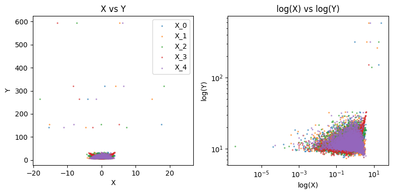
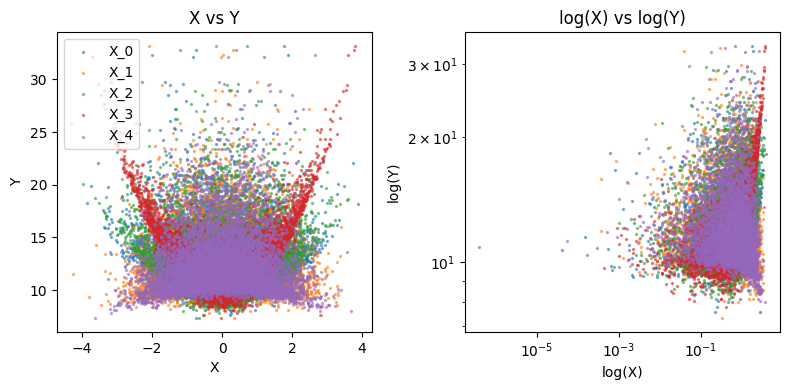
We visualize below each \(X_j\) vs \(Y\) in our training data

../_images/5363e7597d867229f67b829697475668d2d0d92cd1a0eef2d03ba016e959b7ea.png

100-fold CV#

We run k-fold CV over many trials using linear regression. Each k-fold CV trial yields an estimate \(\hat{\text{MSE}} = \text{mean}({\text{MSE}_{CV}}) \approx \text{MSE}_{test}\). Running many trials, we can get a mean and standard deviation of the \(\hat{\text{MSE}}\) estimates, which we compare with the ground truth \(MSE_{test}\)

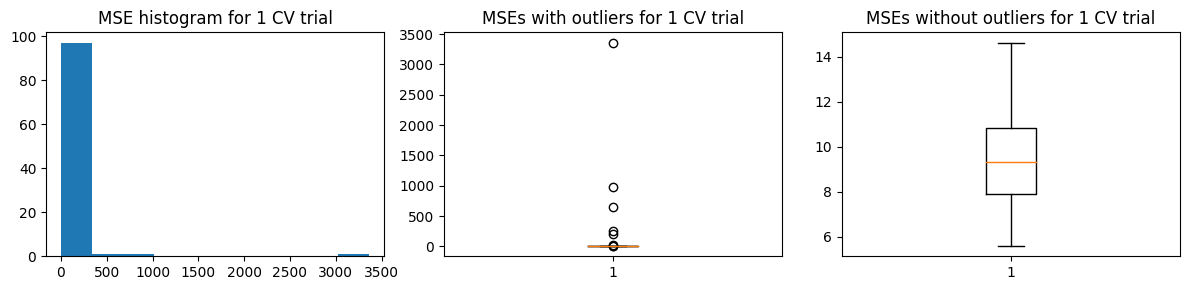
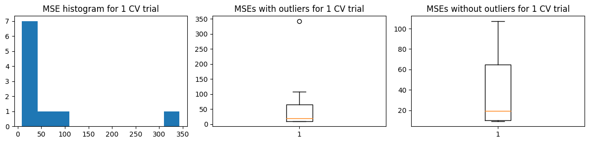
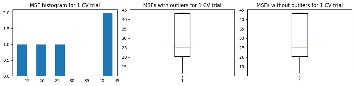
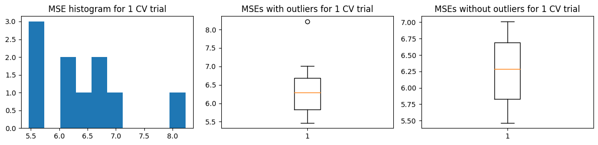
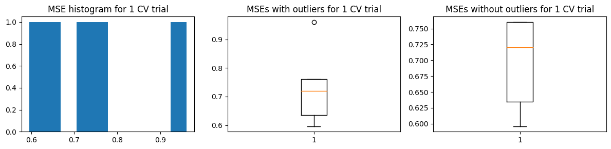
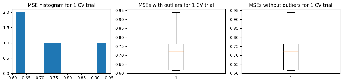
The chart below shows the highly skewed \({\text{MSE}_{CV}}\) values for one trial of k-fold CV. This is due to the presence of high-leverage/outlier points in the training data. But we are not concerned with the distribution of errors in one trial of k-fold CV. We are concerned with the distribution of the estimates \(\hat{\text{MSE}}\)

Show code cell source Hide code cell source

from sklearn import linear_model
from sklearn.metrics import mean_squared_error, r2_score

def run_kfold_trials(k_folds, trials, X_train, Y_train, func, plot=True, seed=42):

    k_folds_idx = np.array(np.split(np.arange(len(X_train)), k_folds))
    mse_means = []
    mse_stds = []

    np.random.seed(seed)
    for trial in range(trials):

        inds = np.arange(len(X_train))
        np.random.shuffle(inds)
        X_train_shuffled = X_train[inds]
        Y_train_shuffled = Y_train[inds]

        mse_list = []
        for k in range(k_folds):

            k_folds_idx_retain = np.delete(np.arange(k_folds), k)
            sample_idx_train = k_folds_idx[k_folds_idx_retain].flatten()
            sample_idx_valid = k_folds_idx[k].flatten()

            X_fold_train = X_train_shuffled[sample_idx_train]
            X_fold_valid = X_train_shuffled[sample_idx_valid]

            Y_fold_train = Y_train_shuffled[sample_idx_train]
            Y_fold_valid = Y_train_shuffled[sample_idx_valid]

            # Create linear regression object
            regr = func

            # Train the model using the training sets
            regr.fit(X_fold_train, Y_fold_train)

            # Make predictions using the testing set
            y_pred = regr.predict(X_fold_valid)

            mse_list += [mean_squared_error(Y_fold_valid, y_pred)]       

        mse_list = np.array(mse_list)    

        # compute the mean MSE from cross validation
        mse_mean = np.mean(mse_list)

        # compute the standard deviation
        mse_std = np.std(mse_list)    

        mse_means += [mse_mean]
        mse_stds += [mse_std]

        if trial == 0 and plot:
            fig, axs = plt.subplots(1, 3, figsize=(12, 3))        
            axs[0].hist(mse_list, cumulative=False)

            axs[1].boxplot(mse_list)
            axs[2].boxplot(mse_list, showfliers=False)

            axs[0].set_title("MSE histogram for 1 CV trial")        
            axs[1].set_title("MSEs with outliers for 1 CV trial")
            axs[2].set_title("MSEs without outliers for 1 CV trial")
            plt.tight_layout()
            plt.show()      
    
    return mse_means, mse_stds

We define 100 k-folds and 100 trials (100-fold each).

../_images/422bb8e96ecd541ee812450474ae8069c023114c520d63cf06aa907c956a6253.png

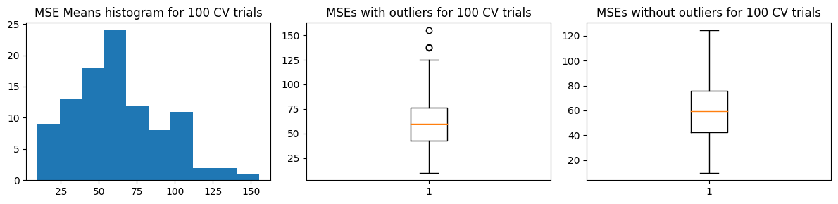
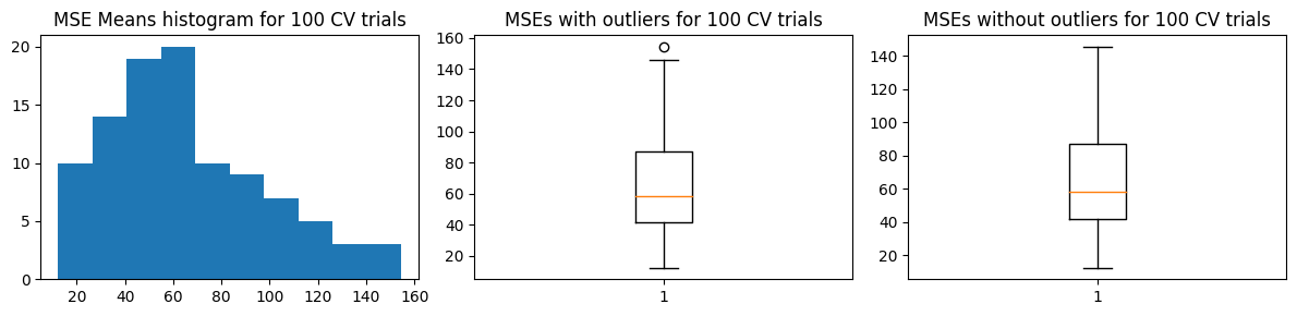
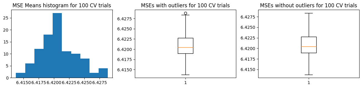
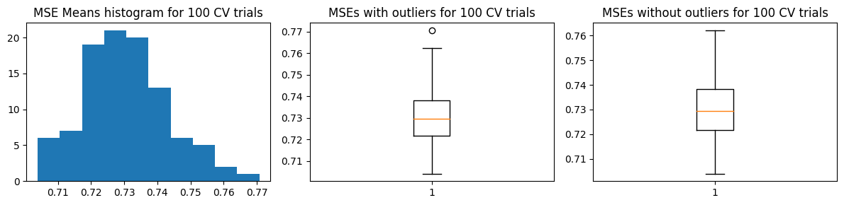
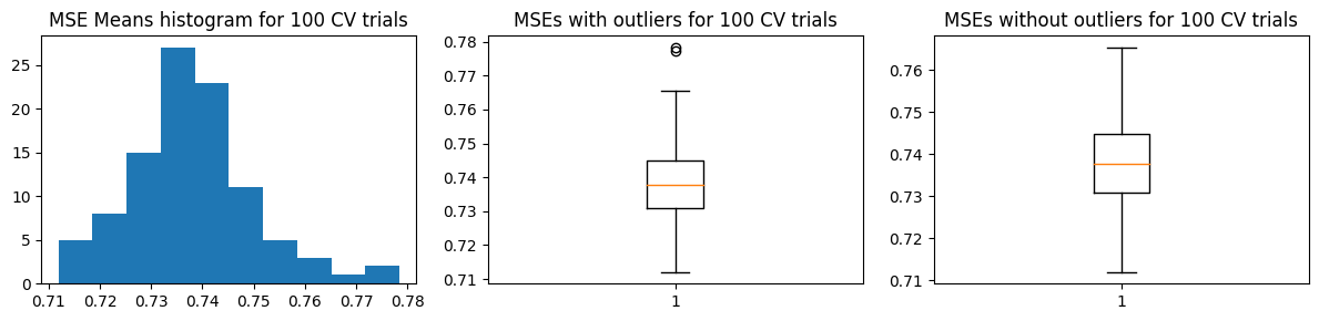
We show below the distribution of \(\hat{\text{MSE}}\) from 100 trials

../_images/9903cef409112f640668aaffebbe4cf4ee1a609788d4fe7c521689278515afa4.png

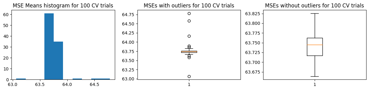
We computed the ground truth \(\text{MSE}_{test}\) as well as the mean and standard deviation of \(\hat{\text{MSE}}\). We find that \(\text{mean}(\hat{\text{MSE}}) \pm \text{std}(\hat{\text{MSE}})\) does not cover \(\text{MSE}_{test}\). However, the estimated \(\hat{\text{MSE}}\) has low variance so it speaks about the consistency of the results when using k-fold CV for this problem.

Mean MSE          63.75660471426123
Std Dev MSE       0.15955756270713287
Ground truth MSE  53.04536320061062

The problem with k-fold CV is if you have rare outliers/high leverage points, it’s possible they get concentrated in one validation fold/group. And this causes the distribution of errors to be highly skewed. Once these points are chosen in one fold, they’re no longer available for the other folds. Thus each k-fold becomes dependent on others, and no longer iid. This violates the assumption of the Central Limit Theorem and prevents us from computing say the standard error properly (which requires iid samples).

How might we go around this? What if instead of regular k-fold, we run a simple train-valid set split but run it 100 times, randomizing each time. With this, we make each validation MSE an iid sample because even if we got datapoints \(X_j, Y_j\) the other “folds” of train-valid splits will still have the chance to select them.

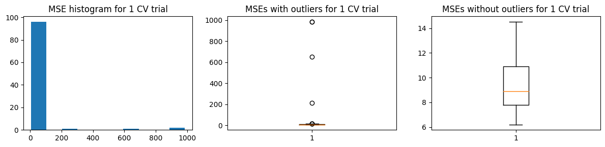
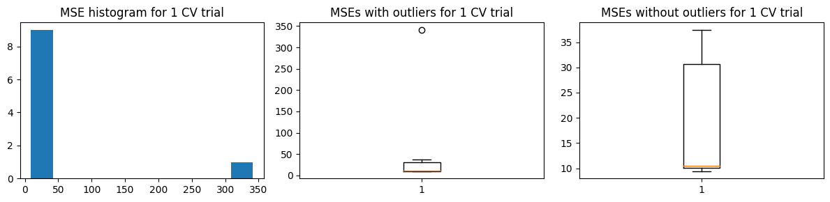
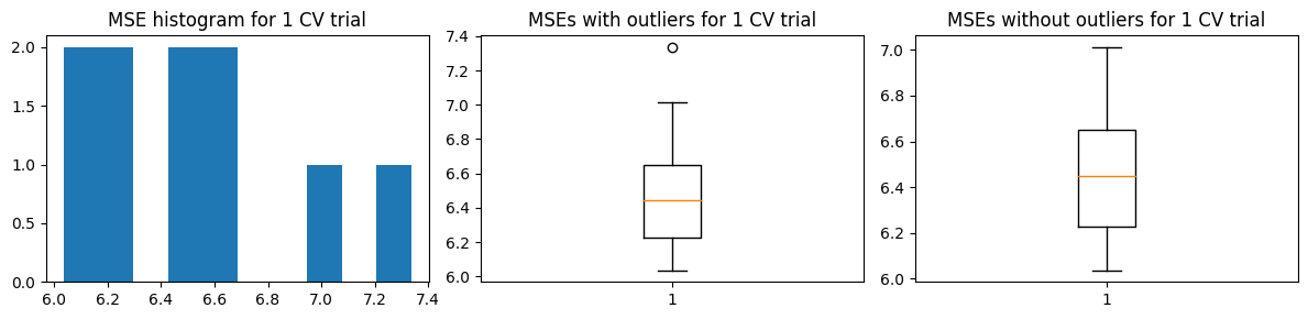
Again, we show below the distribution of \(\text{MSE}_{CV}\) for a single trial (100 validation runs). But we are concerned with the reliability of this estimate, so we run 100 trials.

../_images/f3c37e85b00829e2fd6345f1cf59ab991319d8b16009b7393b76a533d5522070.png

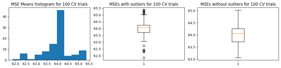
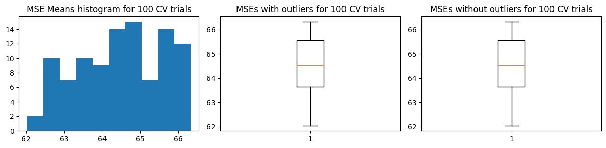
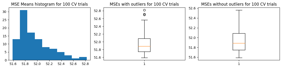
We show below the distribution of \(\hat{\text{MSE}}\) from 100 trials

../_images/420df7c4e69415820e2b426f09dd679e9fe6b5dda72685378eaf7c073cd681a1.png

We find that \(\text{mean}(\hat{\text{MSE}}) \pm \text{std}(\hat{\text{MSE}})\) covers \(\text{MSE}_{test}\). But the increased variance means we expect different results each run of 100-“fold” validation.

Is this approach more reliable than conventional k-fold? How general is this result?

Mean MSE          62.74736033979285
Std Dev MSE       30.408934212115838
Ground truth MSE  53.04536320061062

10-fold CV#

The problem with our experiments above is that our training set is small yet we’re using 100-fold validation. This will make the validation runs correlated since chances are they will share much of the dataset with each other. So now, we experiment on the more realistic 10-fold validation. We still run over 100 trials.

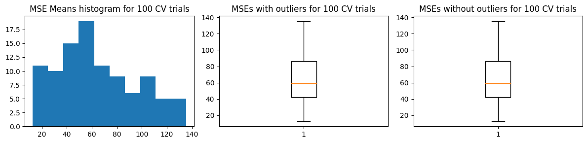
We show below the results of a sample MSE histogram for one trial of 10-fold CV (top charts) and we show the distribution of values of \(\hat{\text{MSE}}\) over 100 trials of 10-fold CV. We find that we get more or less the same result as the 100-fold CV.

../_images/21c52b0811b52cec25129f3666ad3304c4854e8f629e2d882a3a2db55616d4ff.png

../_images/623ccf0c394c8772fd7def3d9a42f6bf0071c8e657b2bd8108b6457b65a5f9a4.png

Mean MSE          63.974719087827445
Std Dev MSE       0.6883531568069371
Ground truth MSE  53.04536320061062

We show the results for the alternative approach. We also get more or less the same results, with some increase in the estimated \(\hat{\text{MSE}}\)

../_images/1f4061073015d27643006d06885c10b79d699a03f4728f389881782b71686d96.png

../_images/2634eb3d15e7085ff4524b0109d71d86a624bf0fcbce5fe7bc394e20d4ab1f50.png

Mean MSE          65.3673539467292
Std Dev MSE       32.5999532851877
Ground truth MSE  53.04536320061062

5-fold CV#

There’s no marked changes when we use 5-fold CV. We show below the results of k-fold CV.

../_images/e942923db301150737569bb08085e0ba083de599a14300da76d2285e27a7a41d.png

../_images/1418ff2b356fbfd59861a2f8e63c848714d09ece70bfdfeb7601b5b5b00b7867.png

Mean MSE          64.47303996932304
Std Dev MSE       1.1310935713605763
Ground truth MSE  53.04536320061062

We show below the results of the alternative approach.

../_images/d078f2b85d273054c27e261dff0dd812f5f22bf7205c962243d24ce057821d3c.png

../_images/dca52f9d4fbad27ef107e5883ee0aab8487ebdb30e0e20f4c7269c0c239fae68.png

Mean MSE          64.03493588943644
Std Dev MSE       31.344888605088617
Ground truth MSE  53.04536320061062

What if no outliers?#

We generate data with no outliers. We find that in both validaation approaches, the test MSE is over-estimated.

Coefficients:                 [ 0.49671415 -0.1382643   0.64768854  1.52302986 -0.23415337]
len(X_train), len(X_test):    10000 990000
len (Y_train), len(Y_test):   10000 990000

../_images/a1aafcf150af48100695e64ea691353e935aeb07297702c9f364a8d687ea290f.png

../_images/d7c7a1d0849f03e209635ca7609c7c3d04e42e282a5d6aae189971f3e28ef8b8.png

../_images/5ec20fa15834fb3f62ca19982db8379114d18c75f4fbbf3e27647931cf7a8fac.png

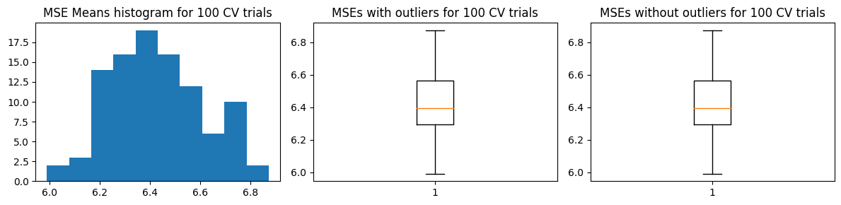
Mean MSE          6.420870371804342
Std Dev MSE       0.00300694628307649
Ground truth MSE  6.108880543132803

Meanwhile the second approach’s standard deviation, relative to its mean, is much lower than when there are outliers. It seems the second approach is more sensitive to the presence of outliers.

../_images/af32303206e6e9abfa85eb390ad4e2f59581ef2a75d568c2b416596a3d5163fe.png

../_images/7393a6a7c9e2364bd32e56e3365764593e626e1c4564f514564aad38117f554a.png

Mean MSE          6.4304134355664315
Std Dev MSE       0.18074357714141273
Ground truth MSE  6.108880543132803

Use in Hyperparameter Tuning#

Without Outliers#

Because linear regression has no hyperparameters, we experiment using kNN regressor instead. We first analyze the dataset without outliers.

Coefficients:                 [ 0.49671415 -0.1382643   0.64768854  1.52302986 -0.23415337]
len(X_train), len(X_test):    10000 990000
len (Y_train), len(Y_test):   10000 990000

It looks like in both validation approaches, the estimated MSE overestimates the ground truth test MSE. However, in terms of selecting the optimal parameter \(k\), the second approach where we do simple validation T times, has more variance in its MSE vs k curves. But it has higher chances of picking the correct \(k\) compared to k-fold CV.

Show code cell source Hide code cell source

from sklearn.neighbors import KNeighborsRegressor
import statistics as st

def hyperparam_run(k_vals, X_train, Y_train, X_test, Y_test, 
                   method='kfold', # kfold or kfold2
                   trials=10, k_folds=5):
    
    fig, axs = plt.subplots(1, 2, figsize=(10, 3))    
    opt_ks = [] # optimal ks
    mse_means_test = []    
    for seed in range(trials):
        mse_means_valid = []    
        for k in k_vals:
            # do standard k-fold cross validation
            func = KNeighborsRegressor(n_neighbors=k, n_jobs=-1)        
            if method == 'kfold':
                mse_means_, mse_stds_ = run_kfold_trials(k_folds, 1, X_train, Y_train, func, plot=False, seed=seed)
            elif method == 'kfold2':
                mse_means_, mse_stds_ = run_kfold2_trials(k_folds, 1, X_train, Y_train, func, plot=False, seed=seed)
            mse_means_valid += mse_means_

            # test mse
            # train on all
            if seed == 0: # just once
                func.fit(X_train, Y_train)
                # Make predictions using the testing set
                y_pred = func.predict(X_test)
                mse_gt = mean_squared_error(Y_test, y_pred)
                mse_means_test += [mse_gt]

        k_min_mse_valid = np.argmin(mse_means_valid)
        opt_ks += [k_min_mse_valid + 1]

        axs[0].plot(k_vals, mse_means_valid) #label='validation')
        axs[0].scatter(k_min_mse_valid + 1, mse_means_valid[k_min_mse_valid], marker='X', c='r', s=100)
    
    k_min_mse_test = np.argmin(mse_means_test)
    opt_k_test = k_min_mse_test + 1
    opt_k = st.mode(opt_ks) # get the most frequent one, which is the likeliest the method will return        
    
    axs[0].set_xlabel("Count Neighbors (k)")
    axs[0].set_ylabel("Mean of MSE")
    axs[0].set_title(f"Validation MSE {trials} Trials | Most likely optimal k = {opt_k}")
                
    axs[1].plot(k_vals, mse_means_test) #label='test')
    axs[1].scatter(opt_k_test, mse_means_test[k_min_mse_test], marker='X', c='r', s=100)
    axs[1].set_xlabel("Count Neighbors (k)")
    axs[1].set_ylabel("MSE") 
    axs[1].set_title(f"Test MSE | Optimal k = {opt_k_test}")       
    plt.tight_layout()

    return opt_k

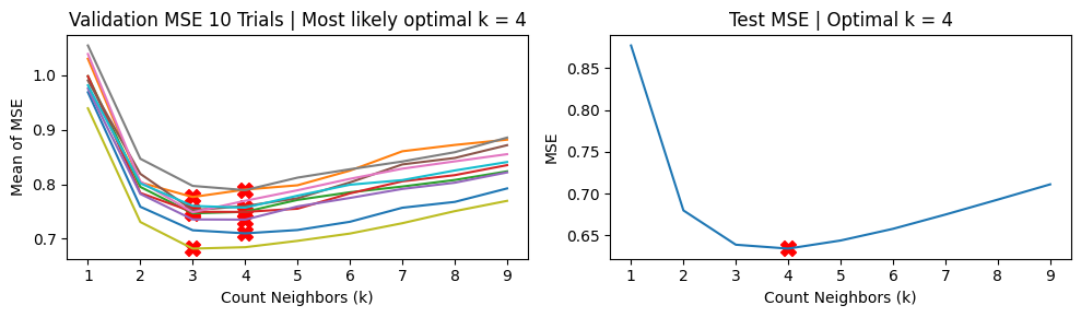
We show the results using 5-fold CV. For the MSE vs k curves, we run 10 trials and indicate the minimum MSE with a red X in each trial (top charts). The middle charts show the distribution MSE per fold from a single trial of validation run, while the bottom charts show the distribution of the estimated \(\hat{\text{MSE}}\) over 100 trials.

We find that \(k=3\) is the likeliest hyperparameter to be chosen, while the ground truth value is \(k=4\).

../_images/74f6bb42a792bc5902a73e56d91a12a8e61e68144774cc6d2039152b7436fbf0.png

../_images/c25a9af33c4233b443fc448ef63c69eefaffc4dfb1a00311a0320e38af275012.png

../_images/2b775a362de785b7d1ee762449c96ee5cad89bcbd7a4eef39283af86309a6cd3.png

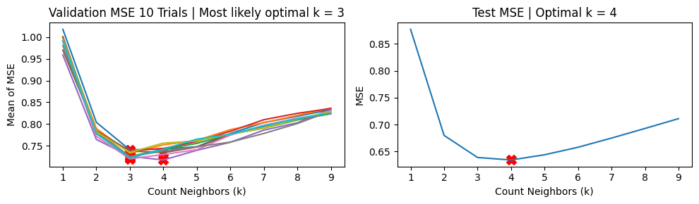
Mean MSE          0.7305736586480543
Std Dev MSE       0.012843940843275855
Ground truth MSE  0.6389746721462332

We show the results using the second approach with 5 “fold” validation runs. For the MSE vs k curves, we run 10 trials of this validation approach, and indicate the minimum MSE with a red X in each trial (top charts). The middle charts show the distribution MSE per fold from a single trial of validation run, while the bottom charts show the distribution of the estimated \(\hat{\text{MSE}}\) over 100 trials.

We find that \(k=4\) is the likeliest hyperparameter to be chosen, which is the same as the ground truth value. However, there are still chances to pick \(k=3\)

../_images/7d7d4efe7610fa106514c12acef6cc30acdfd2bfb751f95a99ff105447fd4010.png

../_images/33873ba270703c0df898ba7fe70c4e58365cd191516db0c522a56ab9cd7ee2fb.png

../_images/f20a7b00bbafbf41d8d92a15a81be87d784439236d0e021b52f107f7da287b06.png

Mean MSE          0.7382083355193587
Std Dev MSE       0.012025683367967064
Ground truth MSE  0.6343301684055197

With Outliers#

Next we analyze the dataset with outliers.

Coefficients:                 [ 0.49671415 -0.1382643   0.64768854  1.52302986 -0.23415337]
len(X_train), len(X_test):    10000 990000
len (Y_train), len(Y_test):   10000 990000

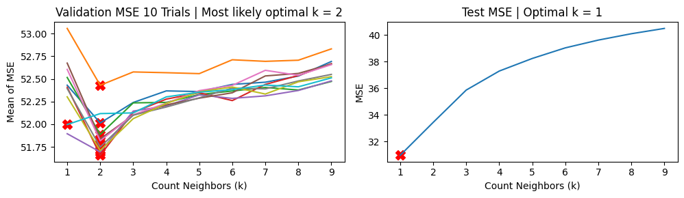
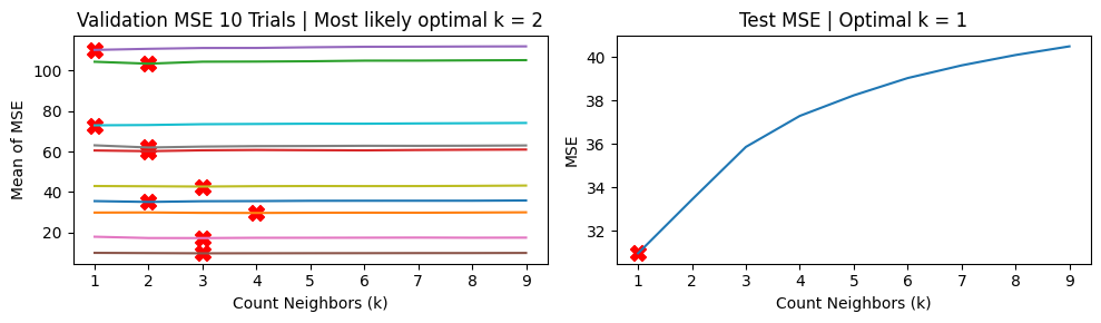
In the presence of outliers, the second approach of T trials of simple validation yields highly variable MSE vs \(k\) curves and can sometimes yield \(k\) values that are widely different from the ground truth optimal value (in this case \(k=1\)).

Meanwhile, k-fold CV yields a more stable set of MSE vs \(k\) curves and mostly returned \(k=2\) and rarely returned \(k=1\). It seems in the presence of outliers, k-fold CV is more reliable.

We show the results using 5-fold CV

../_images/3fdf3a878bddfa3cb4683a2fd365141a996817ba3750bfb90f6d77125dc119c2.png

../_images/571a3907b10c12f79e1ac5ee3782b5efd7df61e6730f4750ec0c61bee41662de.png

../_images/15eb2a0132906c8bfc54a0e2eb69d48c1864fd9b66f65b5d049afffb7b02ad13.png

Mean MSE          51.95621758878725
Std Dev MSE       0.26409296852545755
Ground truth MSE  33.439163683759844

We show the results using the second approach with 5 “fold” validation runs. We note the highly variable MSE vs \(k\) curves.

../_images/e7354dd44e9f56a43108653103871c9206e9171e63548a26d51892a994406ab4.png

Mean MSE          51.95621758878725
Std Dev MSE       0.26409296852545755
Ground truth MSE  33.439163683759844