PCA and Neural Network Autoencoder Connection

We can learn principal component analysis (PCA) linear mapping from D-dimensions of data to M-dimensions of subspace where M < D by using a two-layer autoencoder neural network with linear activation. The model will learn to map from D-space to M-space by minimizing the mean squared error of the reconstruction and the true value.

The intuition why this is the case is because PCA is also a linear mapping that minimizes the mean squared error of the reconstruction of the datapoints from M-space to D-space.

In other words, PCA and a 2-layer neural network autoencoder are practically equivalent.

We load the Wine dataset from Sklearn which has 13 columns that are all float64 and 178 datapoints (rows)

<class 'pandas.core.frame.DataFrame'>
RangeIndex: 178 entries, 0 to 177
Data columns (total 13 columns):
 #   Column                        Non-Null Count  Dtype  
---  ------                        --------------  -----  
 0   alcohol                       178 non-null    float64
 1   malic_acid                    178 non-null    float64
 2   ash                           178 non-null    float64
 3   alcalinity_of_ash             178 non-null    float64
 4   magnesium                     178 non-null    float64
 5   total_phenols                 178 non-null    float64
 6   flavanoids                    178 non-null    float64
 7   nonflavanoid_phenols          178 non-null    float64
 8   proanthocyanins               178 non-null    float64
 9   color_intensity               178 non-null    float64
 10  hue                           178 non-null    float64
 11  od280/od315_of_diluted_wines  178 non-null    float64
 12  proline                       178 non-null    float64
dtypes: float64(13)
memory usage: 18.2 KB

We show below a sample of the dataset

	alcohol	malic_acid	ash	alcalinity_of_ash	magnesium	total_phenols	flavanoids	nonflavanoid_phenols	proanthocyanins	color_intensity	hue	od280/od315_of_diluted_wines	proline
0	14.23	1.71	2.43	15.6	127.0	2.80	3.06	0.28	2.29	5.64	1.04	3.92	1065.0
1	13.20	1.78	2.14	11.2	100.0	2.65	2.76	0.26	1.28	4.38	1.05	3.40	1050.0
2	13.16	2.36	2.67	18.6	101.0	2.80	3.24	0.30	2.81	5.68	1.03	3.17	1185.0
3	14.37	1.95	2.50	16.8	113.0	3.85	3.49	0.24	2.18	7.80	0.86	3.45	1480.0
4	13.24	2.59	2.87	21.0	118.0	2.80	2.69	0.39	1.82	4.32	1.04	2.93	735.0

We then train a neural network autoencoder with linear activation functions that maps 13 input variables to 2 hidden nodes then back to 13 output nodes. The goal is to learn a 2D-mapping from 13D dataset such that we can linearly reconstruct from 2D to 13D with minimal mean squared error. We visualize the network architecture below.

Note that prior to training, we first standard scale the dataset so the values of the variables are comparable.

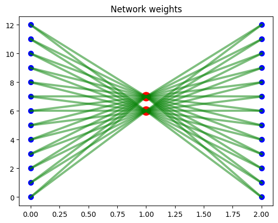
We visualize below the 2D space mapping of the datapoints, predicted vs true values correlation plot of the different variables pooled together, and the network weights over 200 training iterations. We see that the model learns to “spread” the data point projection in 2D space (chart 1).

Once Loop Reflect

<Figure size 640x480 with 0 Axes>

We show below the mapping in 2D space using standard PCA. We see that this projection matches with the projection using the autoencoder above (1st chart above). Although we note that the orientation along the axes are not the same. In other words, the two learned features do not necessarily correspond to the principal axes of PCA, however the learned 2D subspace still matches with the PCA subspace.

Again this is unsurprising because PCA and the linear autoencoder both learn linear mappings that minimize the mean squared error of the projection. They just solve this problem in different ways.