Segregation and Peer Effects#
January 24, 2021
In this notebook we explore
segregation model by Schelling (1971) https://www.stat.berkeley.edu/~aldous/157/Papers/Schelling_Seg_Models.pdf
threshold models by Granovetter (1978) https://sociology.stanford.edu/publications/threshold-models-collective-behavior
Hopefully by doing experiments on these models, we get some new ways of thinking about collective behavior and how outcomes may not necessarily be intuitive by looking at average behaviors.
TLDR#
These are highly simplified models of segregation and how communities of similar individuals tend to form.
For individuals more tolerant of others that are different from them, will they tend to form more “integrated” or mixed communities? How about individuals that are highly intolerant?
Paradoxically, relatively tolerant digital agents tend to want to segregate and form communities of similar individuals. While in some cases, highly intolerant digital agents tend to integrate and form an unstable mixture of different individuals.
These are simplified and do not represent actual people moving around. So it’s definitely something we shouldn’t take too seriously.
However, these are interesting mental models. One takeaway is when you deal with many things interacting with each other, it’s hard to predict what will happen.
Segregation#
Segregation between different people has always been and continue to be an interesting topic. Schelling in his 1971 paper, “Dynamic Models of Segregation” examined the dynamics of segregation via an agent-based modelling approach that led him to interesting insights.
In this section, we will replicate his work. Here are some guide questions for this exercise:
If individuals segregate into highly polarized groups, does that mean that they dislike the other group, e.g. racists or intolerant?
Is it possible for relatively tolerant individuals to form highly-segmented groupings?
If say we have the same population for agents 1 and 2, and they both have a threshold of 20% (they need 20% of their neighbors to be like them for them to be happy), what do you think will be average proportions of like-neighbors per agent?
If the populations of the two agents are not the same, e.g. we have a minority class, what will happen to the segregation patterns and proportions?
What if we limit movement such that agents can only move into vacant areas in their vicinity, how will this affect segregation?
Can we necessarily infer collective behavior from average statistics, e.g. average mixing preference/thresholds?
Can we necessarily infer individual preferences/thresholds from collective behavior?
Segregation in 1D#
Schelling began his model by introducing a 1-dimensional model with two types of agents (black and white) on a line.
Objective - the agents will move into positions that will make all / most of them happy
Rules
From the current positions, an unhappy agent is randomly selected (Schelling selected from left to right)
That agent will them randomly select a vacant position that will make the agent happy
In Schelling’s 1D set up, there were no vacant areas and the agent looks for points between other agents where it can squeeze itself into
Moving into vacant areas on the othat hand is more intuitive because we can think of them as empty houses people move into. You don’t really make your own space by squeezing into two occupied houses.
This rule is applied in Schelling’s 2D model
We repeat until we reach stability (nobody moves) or few people move (if there’s no fixed stability)
Given
p- a fixed proportion of agent 1, agent 2, and empty spaces (houses)n- linear neighborhood (1 dimension) randomly populated by n agents and some empty spacesthresholds- A fixed set of thresholds of the minimum proportion of similar nearby neighbors for each agent that will make them happyk- The distance to the left and right, k, from the agent that defines nearby neighbors. Those at the far left, will have no nearby neighbors to the left and k nearby neighbors to the righttravel_lim- True/False whether we limit the travel to k or not
Impact of Thresholds#
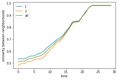
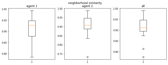
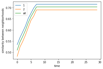
Given k=4, n=70 (Schelling’s params), and equal number of agents, Even if say, we fix at 50% thresholds to be in a neighborhood with similar neighbors (so they will be fine with a mixed neighborhood), they still tend tend to segregate so the average proportion of like neighbors in the vicinity of each agent become ~90% (Schelling saw 81%).
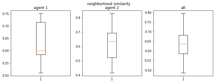
To answer our question above, even if the thresholds are as low as 20% each, the average proportion of like neighbors become 60%-70%. Schelling called these results “striking”
100%|██████████| 30/30 [00:00<00:00, 31.84it/s]
final avg similarities agent 1, agent 2, all 0.980246913580247 0.9833333333333334 0.9816993464052288
100%|██████████| 20/20 [00:00<00:00, 71.15it/s]
Text(0.5, 0.98, 'neighborhood similarity')
100%|██████████| 30/30 [00:01<00:00, 27.65it/s]
final avg similarities agent 1, agent 2, all 0.7146825396825397 0.6895833333333333 0.7028711484593838
100%|██████████| 20/20 [00:00<00:00, 123.82it/s]
Text(0.5, 0.98, 'neighborhood similarity')
Impact of Having a Minority Class#
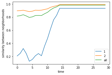
At 50% thresholds for all agents, the median neighborhood similarity for the minority is over 80% (the minority can aggregate) but there are outliers when the minority never aggregates (which is a case when the vacancies are uniformly spread apart)
There is a large variation in outcomes for the minority group, which means the changing the initial state may result in very different outcomes, and hence the equilibrium is not as “stable”
If we make the threshold conservative e.g. 20% for all, we find that the minority does not need to aggregate into one cluster and over 30% similarity is enough though still higher than the 20% value
100%|██████████| 30/30 [00:01<00:00, 27.97it/s]
final avg similarities agent 1, agent 2, all 0.9333333333333332 0.9888888888888889 0.9823529411764707
100%|██████████| 20/20 [00:00<00:00, 102.41it/s]
Text(0.5, 0.98, 'neighborhood similarity')
Travel limits#
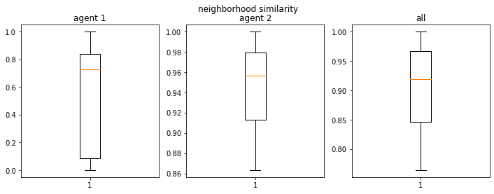
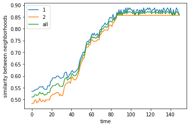
Even if we limit mobility to only the nearest vacant positions, we find that for a given threshold (50%) and proportion (1:1) of agents, we still reach around 80% similarity proportions per agent although convergence is much slower than without travel limits.
Schelling claimed this can be a proxy for “organized movement” where individuals do not move too far apart and thus tend to cluster. He also claimed this can be a proxy for “anticipatory behavior” where agents can only move to nearby areas even if they’re not yet happy, in anticipation of more people coming in.
100%|██████████| 150/150 [00:05<00:00, 28.29it/s]
final avg similarities agent 1, agent 2, all 0.8587912087912088 0.8569444444444444 0.8579047619047618
100%|██████████| 20/20 [00:01<00:00, 17.25it/s]
Text(0.5, 0.98, 'neighborhood similarity')
Segregation in 2D#
The 1D model already gives us insights on “emergent” properties of groups that cannot immediately be inferred from individual dispositions (thresholds). But things get much more interesting when we look at 2D models. Where we can see more interesting patterns. Besides, a 2D model arguably captures reality better since people move in space.
An intuitive way to think about this model is that each cell is a house that’s either empty or occupied by an agent. Agents will then move from house to house in order to reach the set required proportion of nearby neighbors.
Objective - the agents will move into positions that will make all / most of them happy
Rules:
There are two agents who can move around into vacant spaces
Agents are either happy or unhappy
They are happy if the mix neighbors surrounding them are at least as good as desired (threshold)
If they are happy they will stay in their position
Unhappy agents are selected randomly and
Agents belonging to the same class will all have the same threshold, but the two classes may have different thresholds - this was Schelling’s constraint for this exercise
Given
props- a fixed proportion of agent 1, agent 2, and empty spaces (houses)n- the dinemsion of one side of a square neighborhood randomly populated by n agents and some empty spacesthresholds- A fixed set of thresholds of the minimum proportion of similar nearby neighbors for each agent that will make them happythresholds_max- the maximum proportion of like neighbors near an agent (default = None)kernels- the length of a side of a square matrix around an agent to identify nearby neighborstravel_lim- True/False whether we limit the travel to only within a kernel x kernel matrix around the agent or not
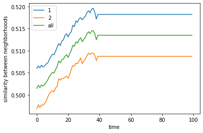
50% demand leads to how much segregation?#
It leads to 90% segregation
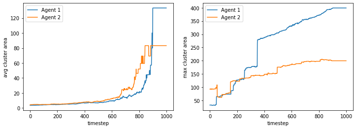
This is a non-intuitive outcome that we see. Despite each individual having only a requirement of 50% similar individuals in the neighborhood, the collective interaction leads to disproportionate segregation. Leading to large clusters of similar neighborhoods.
Our agents are relatively tolerant yet the outcome’s not expected.
100%|██████████| 1000/1000 [00:01<00:00, 649.98it/s]
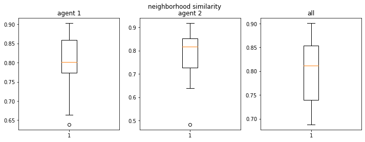
final avg similarities agent 1, agent 2, all 0.9049760447002967 0.9075636736515167 0.9062952280871933
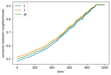
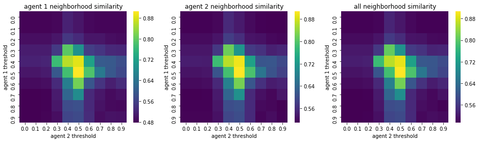
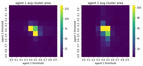
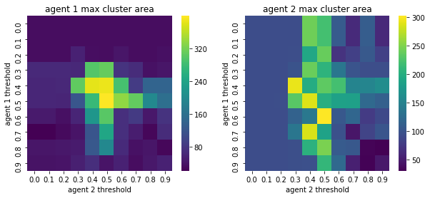
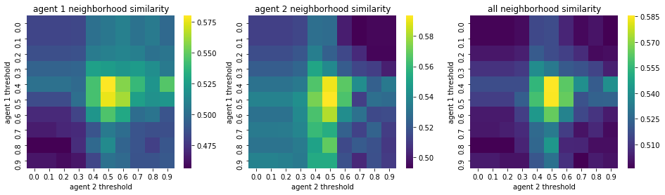
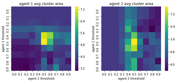
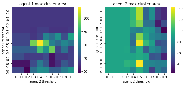
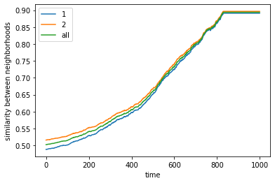
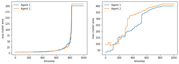
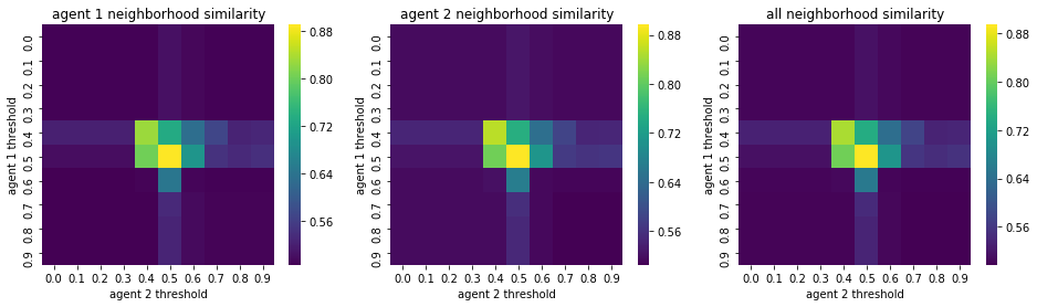
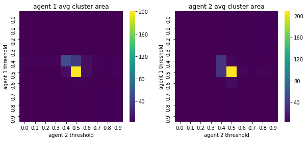
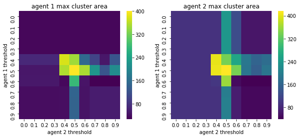
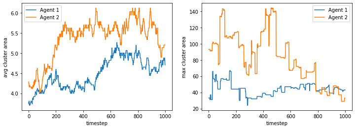
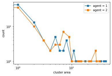
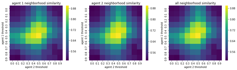
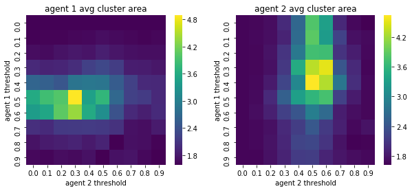
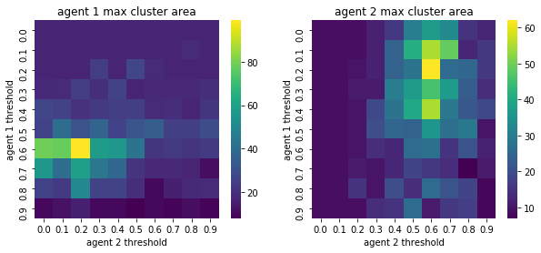
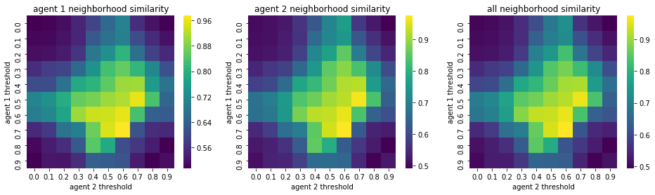
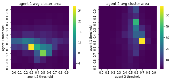
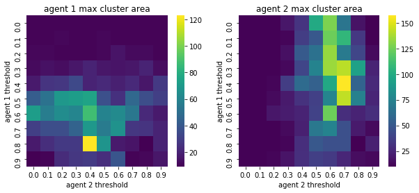
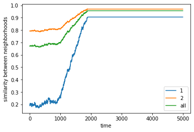
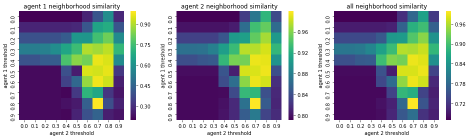
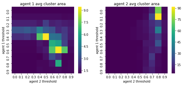
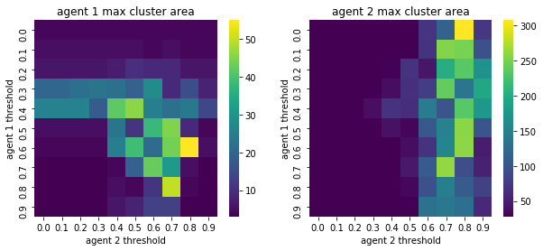
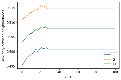
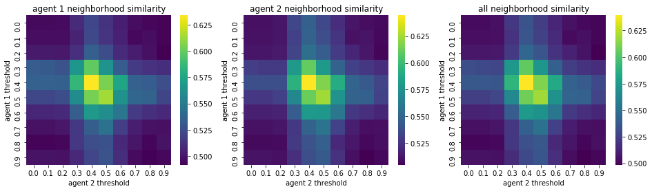
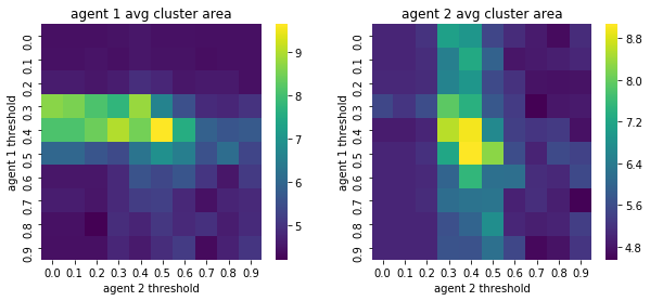
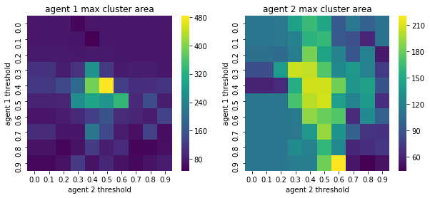
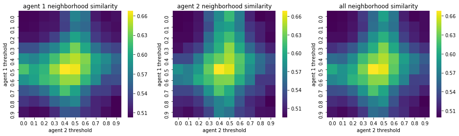
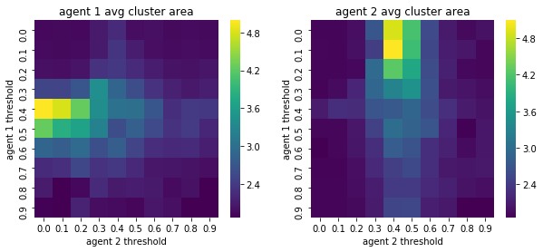
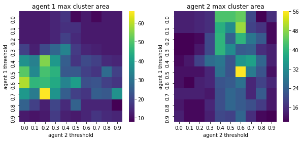
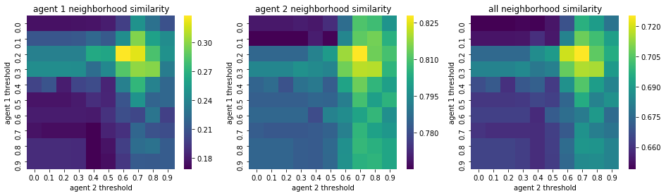
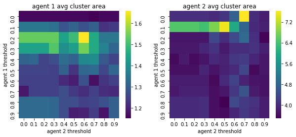
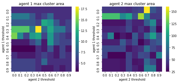
We visualize below the phase spaces showing how the similarity threshold requirements of agent 1 and agent 2 affect neighborhood similarities. We also show how the thresholds affect how large the similar clusters of neighborhoods are. The most segregated neighborhoods come from agents that have ~50% similarity threshold requirements.
What’s interesting is if all agents have 90% similarity requirement, they end up being unsegregated. So less tolerant agents become less segregated or more integrated. That is odd!
We will see in the experiments below what happens when agents are relatively intolerant (requiring 80% of their neighbors to be similar to them)
But first, let’s see what happens if we impose a travel limit on our agents with 50% similarity requirement.
100%|██████████| 10/10 [01:12<00:00, 7.28s/it]
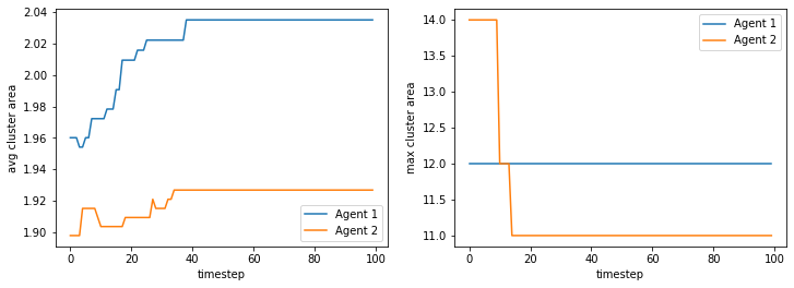
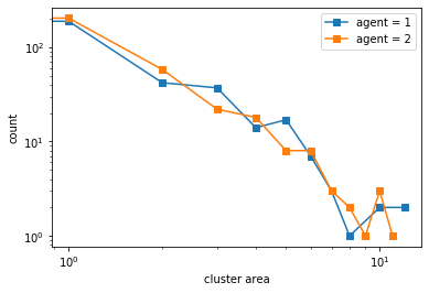
What happens if we impose a travel limit to just the k x k local neighborhood?#
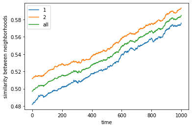
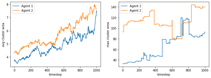
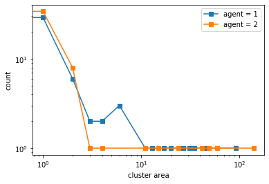
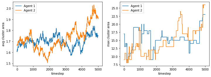
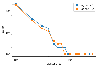
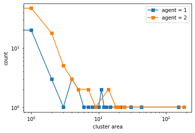
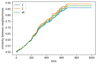
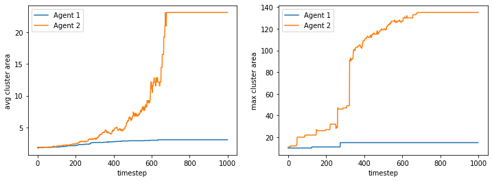
If we limit movement to the kernel size (local neighborhood) at a time, we still get clustering though slower. Here our kernel/local neighborhood is a 5x5 grid.
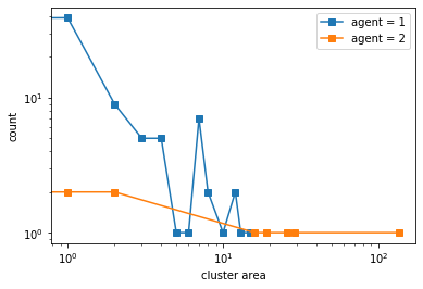
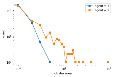
More but smaller clusters tend to form compared to no travel restrictions.
100%|██████████| 1000/1000 [00:01<00:00, 580.43it/s]
final avg similarities agent 1, agent 2, all 0.5759549874488213 0.5934919689215339 0.5848012721460831
We plot the phase spaces.
100%|██████████| 10/10 [01:22<00:00, 8.22s/it]
What if we increase the local k x k neighborhood considered?#
We changed the kernel/local neighborhood to a 13x13 grid around the agent. If an agent’s demand/threshold is based on a larger area, they will tend to form larger clusters
100%|██████████| 1000/1000 [00:02<00:00, 495.61it/s]
final avg similarities agent 1, agent 2, all 0.8910577738738836 0.896696810404354 0.8939325768109861
100%|██████████| 10/10 [02:13<00:00, 13.35s/it]
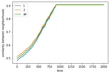
What if we initialized from a semi-clustered initialization and then we run with different parameters?#
We start by allowing the agents to cluster below. We restrict the agent’s movement to a 5x5 grid kernel around it.
100%|██████████| 1000/1000 [00:01<00:00, 512.76it/s]
final avg similarities agent 1, agent 2, all 0.9049760447002967 0.9075636736515167 0.9062952280871933
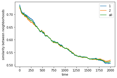
Then we change the local neighborhood/kernel to a 13x13 grid. We notice that this destroys the existing communities and makes it quite difficult to rebuild it. Had the agents started from a random initialization, it would have been quick to form communities (experiments above). But starting from a pre-built community and switching to a different one with different parameters is much harder. This is interesting!
100%|██████████| 2000/2000 [00:02<00:00, 904.46it/s]
100%|██████████| 2000/2000 [00:04<00:00, 450.98it/s]
final avg similarities agent 1, agent 2, all 0.9049760447002967 0.9075636736515167 0.9062952280871933
final avg similarities agent 1, agent 2, all 0.506894464171793 0.5191034455374173 0.5131186507503466
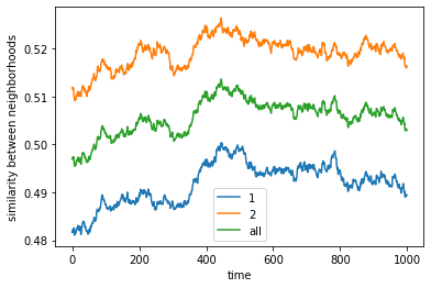
What if agents both have very high demands?#
Now we explore what if agents have very high demands in terms of similarity of agents in their neighborhoods? For example, we try 80% threshold requirement for agent 1 and agent 2. We find that:
It’s hard to find an “equilibrium” if both agents have high demands
This is especially the case if there’s limited free space. And because the agents dont find an equilibrium, they tend to constant move around causing a decrease in segregation.
100%|██████████| 1000/1000 [00:01<00:00, 504.93it/s]
final avg similarities agent 1, agent 2, all 0.48939976715190414 0.5163469525273853 0.5031375479315612
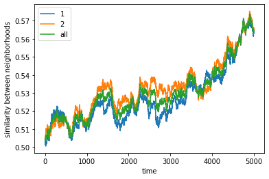
However, if we increase the space, the agents get to a stable state of segregation more easily, but they tend to be highly sparse.
100%|██████████| 5000/5000 [00:21<00:00, 235.43it/s]
final avg similarities agent 1, agent 2, all 0.563269623927012 0.5656334212355428 0.5644585160644388
We show the phase space diagrams
100%|██████████| 10/10 [02:57<00:00, 17.74s/it]
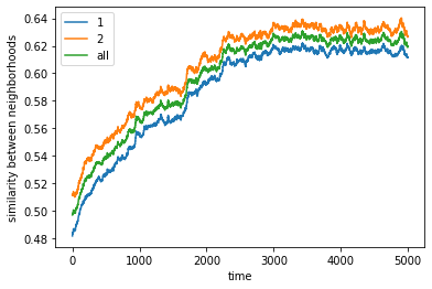
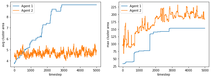
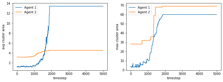
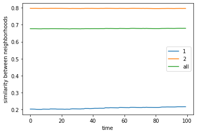
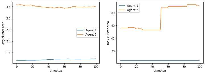
What if the two agent classes have different demands?#
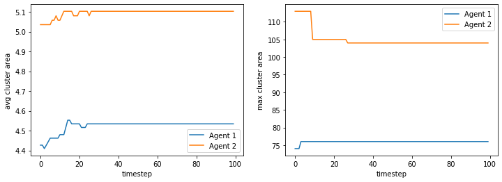
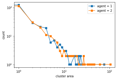
In this case, agent 1 has 30% threshold while agent 2 has 60% threshold
A more demanding group will tend to form more compact clusters than a less demanding group
An equilibrium might be harder to achieve with limited space.
An equilibrium can be achieved faster with a lot of space
100%|██████████| 5000/5000 [00:06<00:00, 824.66it/s]
final avg similarities agent 1, agent 2, all 0.6115512491231043 0.6266706455153158 0.6192591766956044
100%|██████████| 10/10 [01:20<00:00, 8.00s/it]
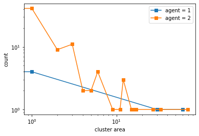
What if we free some space? We find that the more demanding one will have a higher clustering density, as expected.
100%|██████████| 1000/1000 [00:01<00:00, 663.23it/s]
final avg similarities agent 1, agent 2, all 0.8589989355479327 0.8897692453690753 0.874417463896488
100%|██████████| 10/10 [01:13<00:00, 7.32s/it]
What if the demands are the same but the proportions of the classes are different?#
The minority, requiring similar neighbors, will thus cluster together into fewer but more dense clusters. The minority will start from being sparse into larger and larger groups.
Schelling also observed this noting that “The minority tends to accumulate in denser neighborhoods than the majority”
100%|██████████| 5000/5000 [00:05<00:00, 974.34it/s]
final avg similarities agent 1, agent 2, all 0.9049135782865446 0.9689199991652309 0.9558687983786873
100%|██████████| 10/10 [01:10<00:00, 7.04s/it]
Integrationist Preferences#
Here, we add a limit to the maximum proportion desired around the agent, meaning, the agent does not like if say > X% of the neighborhood is similar to it. In this case, we define our threshold to be between 20% to 90% similar.
We observe some aspects that Schelling also observed
Schelling noted “More individuals may be incapable of being satisfied” or an equilibrium is harder to reach
If there is a minority, they are “rationed” or shared among the majority members. Thus no big clusters form
It might seem that segregation is much more “static” or “stable” than integration
100%|██████████| 100/100 [00:03<00:00, 30.63it/s]
final avg similarities agent 1, agent 2, all 0.50076872921975 0.5145692112651683 0.507739100840569
100%|██████████| 10/10 [02:40<00:00, 16.03s/it]
If we make the agents sparse and allow for more empty space, an equilibrium is reached where the two agent classes are integrated with one another, with little clumping or clustering of similar agents.
100%|██████████| 100/100 [00:03<00:00, 31.49it/s]
final avg similarities agent 1, agent 2, all 0.5182092538592996 0.5087099110627543 0.5134857411548018
100%|██████████| 10/10 [03:01<00:00, 18.19s/it]
Even if we add more space, if there is a minority, they will be “rationed” among the majority so the minority will keep switching places.
100%|██████████| 100/100 [00:03<00:00, 28.52it/s]
final avg similarities agent 1, agent 2, all 0.21644608470104487 0.7961650148914287 0.6789441139796044
100%|██████████| 10/10 [03:07<00:00, 18.72s/it]
Bounded Neighborhood Model#
This model sets a fixed boundary for a sub-neighborhood. Everyone is concerned about the color ratio inside the sub-neighborhood and make their decision based on this value. We can interpret this model as being analogous to becoming part of a physical space or organization e.g. a restaurant, company, school, or even riots (Granovetter).
Here, Schelling introduced the concept of “tolerance” which is the proportion of same agents in the sub-neighborhood. Granovetter will later on expand on this concept which he would call “threshold.”
In this variation of the model, Schelling introduced the possibility of each agent having different thresholds from each other. He further analyzed how the distributions of thresholds affect the stability and outcomes of the system i.e. proportions of agents in the sub-neighborhood.
Here, agents can move out or move in depending on the proportion of like-agents in the sub-neighborhood. Movement is ordered by lowest threshold breached.
Objective - the agents will move into positions that will make all / most of them happy
Rules:
There is/are a predefined neighborhood/s with set boundaries, we’ll refer to as subneighborhoods
There are two agents who can move into and out these subneighborhoods
They stay in the neighborhood if the mix neighbors inside the neighborhood are at least as good as desired (threshold)
Agents leave the subneighborhood if the proportion of neighbors are no longer preferred
Agents move one by one and the order by which agents leave or enter based on their preferences (thresholds)
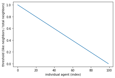
Individual agents may have different thresholds following some predefined function - in this case, a linear function with thresholds from 100% (all like-neighbors needed) to 0% (no like neighbors needed)
Threshold distributions may be different for the two agents - but for this exercise, we assume them to be the same
Given
props- a fixed proportion of agent 1, agent 2, and empty spaces (houses)n- the dinemsion of one side of a square neighborhood randomly populated by n agents and some empty spaces
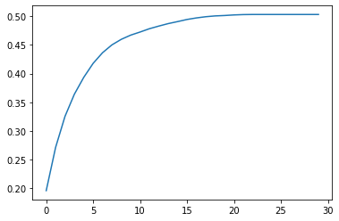
We define below the function that determines the threshold of each agent. We define a smooth line from 100% to 0% and each agent will have a unique value in that range.
Text(0, 0.5, 'threshold (like neighbors / total neighbors)')
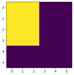
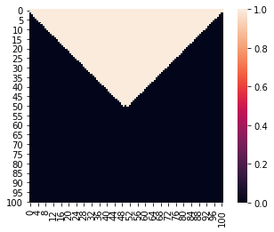
We define below the fixed subneighborhood. Yellow is the subneighborhood (imagine a town), and the dark magenta is outside the subneighborhood.
<matplotlib.image.AxesImage at 0x7faba9a75390>
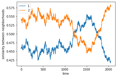
What happens if there are the same number of agents 1 and agents 2?#
complete
final avg similarities agent 1, agent 2  0.43434343434343436 0.5656565656565656
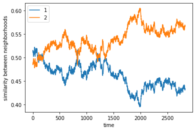
We run another trial of the configuration above.
complete
final avg similarities agent 1, agent 2  0.4208754208754209 0.5791245791245792
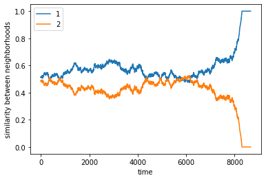
What if the numbers of agent classes are slightly imbalanced?#
The minority will tend to occupy the subneighborhood.
complete
final avg similarities agent 1, agent 2  1.0 0.0
What if we have multiple neighborhoods?#
For the same proportions of agents 1 and agents 2, segregation easily arises.
complete
final avg similarities agent 1, agent 2  0.0 1.0
Threshold Models#
Thresholds from Plots#
We can now define a threshold function that is non-linear like in the distribution below, which is a truncated cumulative distribution function of an exponential distribution
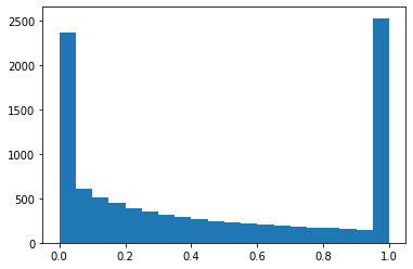
Text(0, 0.5, 'cdf - prop. of population having <= threshold')
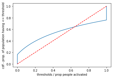
How can we find the equilibrium from these plots?#
Intuitively, we have a sense that the system is in equilibrium if the previous proportion of people is the same as the next proportion
Analytically, that means that the proportion at time t \(r(t) = r(t+1)\)
Visually, we can plot from an initial proportion on the x-axis upwards to find the proportion of population with <= threshold, then we can move to the 45 degree line, and back to the CDF, and so forth until we reach a stable point. The rationale is: if there are currently, 60% (x axis) activated and 80% (y-axis_ have thresholds less than or equal that, they will have to activate (move horizontally to an x-axis proportion equal to the y-axis value) and so on.
Observations of Equilibrium Points from Plots Below#
For exponential distributions, we may find a stable equilibrium at a certain point between 0% and 100% activated
For a normal distribution, equilibria tend to be either 0% or 100% activated
Exponential Distribution#
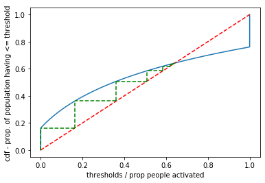
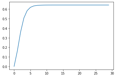
In the cellular automata model below, we start with 0% activated. We find that the proportion of activated grows until it becomes ~60% as we have computed above.
charts/threshold/1_dist_exp_r0_0.0/ exists
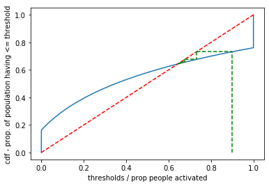
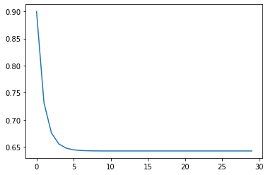
If we start with 90% of the population activated, the number of activated declines until we reach only ~60% activated, which again, is the stable equilibrium.
charts/threshold/1_dist_exp_r0_0.9/ exists
Normal Distribution#
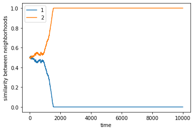
We not investigate a threshold using the cumulative distribution function (CDF) of a normal distribution. From our analysis below, we expect either 100% activation or 0% activation depending on the starting point.
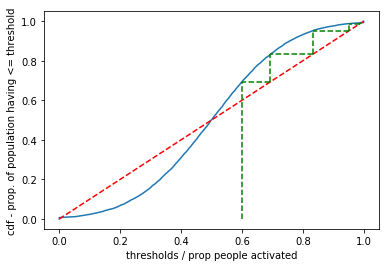
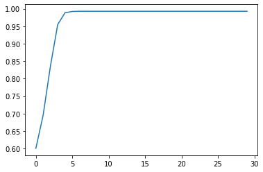
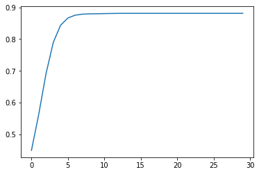
Based on the cellular automata simulation, we find that the proportion of activated goes to 100% if we start with 60% activated.
charts/threshold/1_dist_norm_r0_0.6/ exists
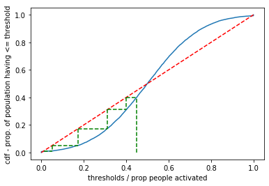
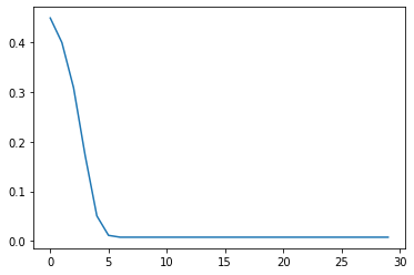
Based on the cellular automata simulation, we find that the proportion of activated goes to 0% if we start with 45% activated.
charts/threshold/1_dist_norm_r0_0.45/ exists
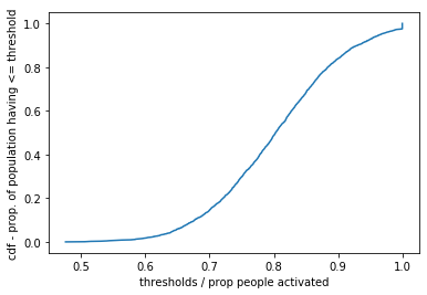
Inverse Normal Distribution#
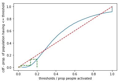
Now let’s look at a threshold based on the inverse normal distribution.
thresh = inv_norm_dist(props, mean=0.5)
plt.plot(thresh, props)
plt.plot([0, 1], [0, 1], 'r--')
r1 = 0.2 # proportion at time t
r0 = 0
for i in range(10):
r2 = sum(thresh <= r1) / len(thresh) # how many people will activate
plt.plot([r1, r1], [r0, r2], 'g--')
plt.plot([r2, r1], [r2, r2], 'g--')
r1 = r2 # r1 is the new r2
r0 = r2
plt.xlabel('thresholds / prop people activated')
plt.ylabel('cdf - prop. of population having <= threshold')
plt.show()
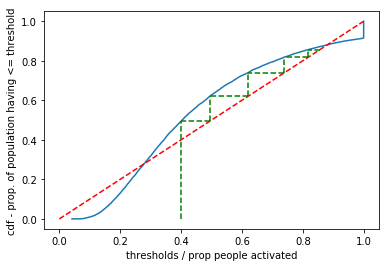
plt.plot(thresh, props)
plt.plot([0, 1], [0, 1], 'r--')
r1 = 0.4 # proportion at time t
r0 = 0
for i in range(5):
r2 = sum(thresh <= r1) / len(thresh) # how many people will activate
plt.plot([r1, r1], [r0, r2], 'g--')
plt.plot([r2, r1], [r2, r2], 'g--')
r1 = r2 # r1 is the new r2
r0 = r2
plt.xlabel('thresholds / prop people activated')
plt.ylabel('cdf - prop. of population having <= threshold')
plt.show()
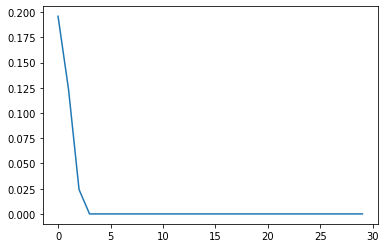
# visualize with cellular automata model

props = np.arange(0, 1, 1/(n**2)) # agents are indices, value is the (cumulative proportion)
thresh = inv_norm_dist(props, mean=0.5)

r1 = 0.2 # initial activated population
seed = 1
np.random.seed(seed)
neighborhood = np.random.choice([0, 1], size=n*n, p=[1-r1, r1]).reshape((n, n))

new_dir = f'charts/threshold/{seed}_dist_norm_r0_{r1}/'

rs = run_thresh_sim(neighborhood, props, thresh, new_dir)
plot_thresh_gif(new_dir)
plt.plot(rs)
plt.show()
charts/threshold/1_dist_norm_r0_0.2/ exists
# visualize with cellular automata model

props = np.arange(0, 1, 1/(n**2)) # agents are indices, value is the (cumulative proportion)
thresh = inv_norm_dist(props, mean=0.5)

r1 = 0.45 # initial activated population
seed = 1
np.random.seed(seed)
neighborhood = np.random.choice([0, 1], size=n*n, p=[1-r1, r1]).reshape((n, n))

new_dir = f'charts/threshold/{seed}_dist_norm_r0_{r1}/'

rs = run_thresh_sim(neighborhood, props, thresh, new_dir)
plot_thresh_gif(new_dir)
plt.plot(rs)
plt.show()
charts/threshold/1_dist_norm_r0_0.45/ exists
Stability of Equilibrium vs Threshold#
We test the stability of the equilibrium if we modify our thresholds a bit so that the mean stays the same but the standard deviation differs
Even if our mean stays the same at 0.5, varying the standard deviation of thresholds varies the point at which the system reaches equilibrium
The implication of this is we should be wary of merely looking at averages (say the average individual) to explain collective phenomena.
Text(0, 0.5, 'equilibrium proportion')

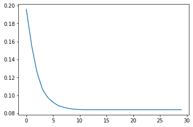
We visualize the results above for standard deviation = 0.3 and equilibrium point ~ 0.08.
charts/threshold/1_dist_norm_r0_0.2_0.3/ exists
We visualize the results above for standard deviation = 0.5 and equilibrium point ~ 0.5.
charts/threshold/1_dist_norm_r0_0.2_0.5/ exists
Standing Ovation Problem#
Here’s a modification of Granovetter’s activation model. We incorporate some rules that intuitively exist when we’re simulating a standard ovation after a performance. These rules are:
Objective - simulate a standing ovation process
Rules
The audience only sees agents within a field of view. The implications are:
Those at the front may have the least information about the true proportion of activated users
Those at the far back may have the greatest information
Agents have a defined field of view that can be patterned after some shape e.g. cone-shaped
The audience can be heterogenous
Like in Schelling’s and Granovetter’s models, we can apply a threshold value to indicate
the proportion of agents perceived to activate that will cause an agent to activate.
the threshold for the quality of the performance
We will follow Miller and Page’s model where the quality threshold is fixed at 0.5
Agents cannot switch seats
Agents can change decisions based on new information
The agent stands up based on some factors
Each agent assesses (here, randomly generated) the quality of the performance
If the quality exceeds the agent’s threshold the agent stands up
The agent who stands up from quality will remain standing
At t+1 onwards, agents will decide whether to stand up or not based on the proportion of agents standing up that they see
“Synchronous” updating is used - per time step, all agents whose thresholds are breached all stand up (or sit down)
Notes: Our quality assessments and threshold for peer-pressure are drawn from a normal distirbution given mean and standard deviation as parameters
Parameters
n- for an n x n matrix representing audienceq_thresh- quality threshold exceeding which means the agent will stand up no matter what (one threshold for all users)kernel- the field of view of each agent indicated by zeros and ones on an m x m matrixp_mean- the mean of a normal distribution of peer-pressure thresholdsp_stdev- the standard dev of a normal distribution of peer-pressure thresholdsq_mean- the mean of the normal distribution of performance quality assessmentsq_stdev- the standard deviation of the normal distribution of performance quality assessments
We’d like to check:
Is it possible for majority to stand up even if most agents did not like the performance?
Stable equilibrium, i.e. proportion standing up
Number of iterations before reaching the stable equilibrium
Proportion of agents standing over time or the reverse: “Stick in the Muds” - proportion of people that did the opposite of the majority at steady state
Below is each agent’s cone of vision. The agent sees others in the bright triangle or cone of vision in front of it.
We then define the “peer pressure” threshold parameters to be the CDF of a normal distribution. There’s one threshold for peer pressure and another for how they assessed the play.
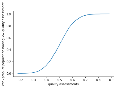
sanity check prop people having thresh < 0.6 0.0172
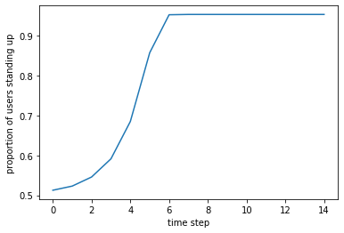
We show the evolution of proportion of people who do the standing ovation. Peer pressure plays a huge role.
sim complete
Text(0, 0.5, 'proportion of users standing up')