Distribution of the Sum of Random Variables vs Sum of Distributions#
\(p(x + y) \) - The distribution (or density) of the sum of states of two random variables \(X\) and \(Y\)
\(p(x) + p(y)\) - The sum of two distributions/densities
\(p(x + y) \neq p(x) + p(y)\)
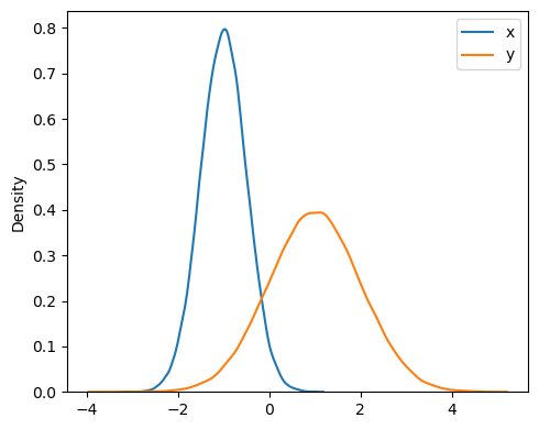
We generate \(N\) random states/samples for two independent random variables \(X\) and \(Y\) that follow two Gaussian distributions with different means and standard deviations.
Show code cell source
import numpy as np
import matplotlib.pyplot as plt
from scipy.stats import norm
import seaborn as sns

# Inputs
N = 100000 # number of random samples
mu_1 = -1 # mean of X
mu_2 = 1 # mean of Y
sigma_1 = 0.5 # std of X
sigma_2 = 1 # std of Y

x = np.random.normal(mu_1, sigma_1, size=N)
y = np.random.normal(mu_2, sigma_2, size=N)

plt.figure(figsize=(5, 4))
sns.kdeplot(x, label='x')
sns.kdeplot(y, label='y')
plt.legend()
plt.tight_layout();
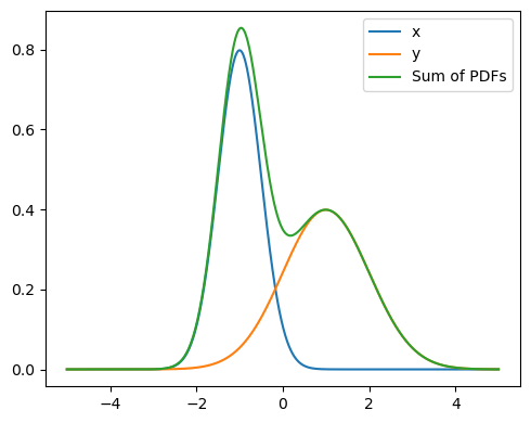
We show the sum of the densities below \(p(x) + p(y)\). It has two peaks and is clearly not a Gaussian distribution.
Show code cell source
x = np.linspace(-5, 5, N)
pdf1 = norm.pdf(x, mu_1, sigma_1)
pdf2 = norm.pdf(x, mu_2, sigma_2)

# Add PDFs
pdf_sum = pdf1 + pdf2

plt.figure(figsize=(5, 4))
plt.plot(x, pdf1, label='x')
plt.plot(x, pdf2, label='y')
plt.plot(x, pdf_sum, label='Sum of PDFs')
plt.tight_layout()
plt.legend()
plt.show()
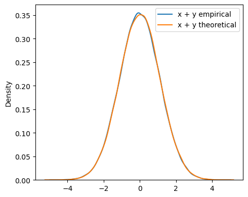
Meanwhile below is the density of the sum of states \(x\) and \(y\) of random variables \(X\) and \(Y\): \(p(x+y)\). The resulting density is also a Gaussian distribution, \(p(x + y) =\mathcal{N}(\mu_1 + \mu_2, \sigma_1^2 + \sigma_2^2)\). We show below the alignment between the empirical density and theoretical density.
Show code cell source
# sum of variables
z = np.random.normal(mu_1, sigma_1, size=N) + np.random.normal(mu_2, sigma_2, size=N)

plt.figure(figsize=(5, 4))
sns.kdeplot(z, label='x + y empirical')

# The theoretical value
mu_3 = mu_1 + mu_2
sigma_3 = np.sqrt(sigma_1**2 + sigma_2**2)
z = np.random.normal(mu_3, sigma_3, size=N)
sns.kdeplot(z, label='x + y theoretical')
plt.legend()
plt.tight_layout();